Chapter 18
Virtual pre-zygotic, post-zygotic and combined curves square well with reality.
Ovum and sperm combine to form a zygote, which is a single cell that goes on to form an embryo and then fetus and certain tissues that will support the pregnancy. Anything that prevents that formation of a zygote is “pre-zygotic” infertility, while anything that prevents the pregnancy at the zygote stage from going on to have offspring is “post-zygotic.”
Since this is a cyclic process the question inevitably arises, “When does a post-zygotic process of one generation become a pre-zygotic process of the next?” or, “If I can’t get a date, is that pre- or post-?” For me, the moment is when the sperm makes physical contact with the ovum. Anything before that instant is post-zygotic from the prior generation. If somebody has a different opinion, I am certainly interested in listening. On the other hand, spend a few minutes looking back over the source code and you will see that in the computer program, the two are not different facets of the same process. They do not occur together during the creation of a new generation.
Intuitively, one might expect that pre-zygotic should precede post-zygotic, but when I am thinking about it, I generally consider post-zygotic first and so we shall. We’ll have to go back to source code. An orderly mind might put all computer related material together, but except for a few grandmaster geeks, that would be reader abuse.
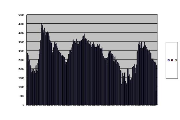
How does the post-zygotic form of infertility do at predicting the known Sibly curve? Here, figure 53, is a graph of a number of runs comparing the virtual reproductive rate with virtual population size under the influence only of post-zygotic outbreeding infertility.
Vertical axis on the left is offspring per member of the population and horizontal axis the maximum population size. Runs last up to 1,000 generations. Methylation rate 1,500 per site per 100,000 generations. One unit of methylation mismatch loses 1,500 one thousandths of an offspring.
Fig. 53
The most basic distinction in infertility is between pre-zygotic infertility in which the sperm is unable to unite with the ovum and post-zygotic infertility in which the zygote does not develop into a fully fertile adult. Both of these can be modeled by a computer program that shows infertility in a population. Figure 53 shows offspring against maximum population size. Notice how closely it resembles figure 22 in chapter 4, which shows in Iceland the number of grandchildren graphed against kinship of a couple and which we interpreted to represent post-zygotic infertility. At very low population sizes, there is a rapid fall in fertility with increasing kinship, much like the obvious inbreeding depression shown in graph 23, chapter 5, using Danish data graphing fertility against what they call marital radius.
Now the cause of inbreeding depression becomes clear. Inbreeding depression in and of itself confers no advantage and obvious disadvantage. It should have long since been eliminated by selection. But it is an inescapable consequence of outbreeding depression, which is vital to long term survival of a species. Indeed selection might have eliminated post-zygotic outbreeding depression and relied solely on pre-zygotic outbreeding depression, but this would have entailed given up the opportunity of importing valuable genes from elsewhere in the species. So instead, selection gives us vigorous outbreeding infertility, apparently by multiple mechanisms such as falling sperm counts, shrinking penis size, behavioral social changes that are not reproductively productive and possibly autism spectrum disorder.
Next is figure 54, which shows a computer simulation of a population limited only by pre-zygotic outbreeding depression.
A virtual population controlled only by pre-zygottic infertility. The vertical axis is fertility and the horizontal axis is population size, essentially the same as figure 53. Notice the lack of inbreeding depression.
Fig. 54
The axes, fertility on the vertical axis against maximum population size on the horizontal axis, are virtually the same as in figure 53. There is no inbreeding depression. I do not know what to make of the point at the origins of the axis. I believe the population size must be limited to one, which is the end of the line for any animal population. Notice how well this matches figure 21 in chapter four. That shows fertility against kinship as reckoned from the extensive Iceland genealogy. Both show a remarkable absence of inbreeding depression. The match is better than we had any right to hope for.
Somehow pre-zygotic infertility “saturates;” it reaches a point, well short of total infertility where it has done all the damage it can do.
In order better to reflect reality, it might be good to tweak the source code I have shown you. Or maybe not. Feel free to ignore what follows in braces: {Find the place where the program goes (Bold type):
PreZInfertility = 0;
Loss = PreZImpact * MisMatch;
if(Loss >= 1000)
{//32a Lower fertility one offspring at a time
while(Loss >= 1000)
{//33
PreZInfertility = PreZInfertility +1;
Loss = Loss - 1000;
}//33
}//32a Lower fertility one offspring at a time
else
{//32b No whole offspring lost
}//32b No whole offspring lost
coin = rand();
Coin = coin % 1000;
if(Loss > Coin)
{//34a Lose fractional offspring
PreZInfertility = PreZInfertility + 1;
}//34a Lose fractional offspring
else
{//34bKeep fractional offspring
}//34b Keep fractional offspring
OffspringComing = OffspringComing - PreZInfertility;
}//29a PreZsites > 0
else
{//29b PreZsites = 0
}//29b PreZsites = 0
//Now we don’t want OffspringComing (if that’s not self-explanatory, look it up in the program) to drop below 2 on the basis of pre-zygotic infertility alone. So we’ll say:
if(OffspringComing < 2)
OffspringComing = 2;
//And stick it in here ):
PreZInfertility = 0;
Loss = PreZImpact * MisMatch;
if(Loss >= 1000)
{//32a Lower fertility one offspring at a time
while(Loss >= 1000)
{//33
PreZInfertility = PreZInfertility +1;
Loss = Loss - 1000;
}//33
}//32a Lower fertility one offspring at a time
else
{//32b No whole offspring lost
}//32b No whole offspring lost
coin = rand();
Coin = coin % 1000;
if(Loss > Coin)
{//34a Lose fractional offspring
PreZInfertility = PreZInfertility + 1;
}//34a Lose fractional offspring
else
{//34bKeep fractional offspring
}//34b Keep fractional offspring
OffspringComing = OffspringComing - PreZInfertility;
if(OffspringComing < 2)
OffspringComing = 2;
}//29a PreZsites > 0
else
{//29b PreZsites = 0
}//29b PreZsites = 0
You might have to play around with that “2” a bit. Or maybe you can come up with a better logic. }
The moment has come to leap into population experience simulations based on the source code that includes both pre-zygotic and post-zygotic processes. There are a number of patterns that might emerge.
The first pattern we might see is a low, constant population such as the Australian mice usually show, as if figure 42, chapter 15. That is a sort of a skeleton in my closet. I have not been able to produce such a behavior with a virtual population although I have not pursued it with much vim. I am discouraged from the attempt because of the very noisy quality of my results. Remember the noisy quality shown in figure 42, chapter 15. Using the computer at which I now sit, I could in theory add random access memory until the size of the compiled program in random access memory increased by a factor of 100. I would expect that if the number of sites available for methylation were increased that much and the rest of the program tweaked appropriately, it would drive the noise level down by a factor of 10. That just might be enough to clean the output up to the point where a low, stable population could exist. Feel free to try it yourself, but I have taken it on the chin from programing so often, I think I must pass. A pattern I do find is damped oscillation, such as that shown by my fruit flies and by European voles. I found a combination of parameters that seems to fill that bill. Graphing offspring on the vertical axis against successive generations on the horizontal we get figure 55:
Graph of a run of a virtual population, generations on the horizontal axis and offspring on the vertical. It is noisy but shows damped oscillation.
Fig. 55
This curve was obtained with a run in which only 200 of a saved population were brought out and run; all other conditions were highly tweaked. This is an ungainly example, but it can, indeed, be seen in wild voles, as we have seen, and in captive fruit flies. As lest so far as our data goes, these animals never exhibit any other pattern although they have the opportunity. This pattern is a winner. I have never seen it in a population that went extinct.
A second pattern is the double peak, or as we more specifically call it, strengthening oscillation. It is shown in figure 56.

Graph of a run in which conditions were identical with those of figure 55 except that maximum population was permitted to rise higher, to 3,000. As before, offspring are on the vertical axis and generations on the horizontal. There is strengthening oscillation leading to extinction.
Fig. 56
We have seen this strengthening oscillation in the survival of civilizations and dynasties, in the farmers of Long House Valley, and in wild mouse populations in Australia. None of these, neither human nor murine, showed damped oscillation in spite of ample opportunity. This pattern is a loser. Extinction always supervenes in the cases we have seen.
A final pattern is a single peak and a crash. I did another run letting the maximum population rise to 4,000, but otherwise kept conditions identical with figures 55 and 56, which is show in figure 57.

Another run with parameters the same as figures 54 and 55 except that population was permitted to rise to 4,000 offspring. Number of offspring is on the vertical axis and generation on the horizontal.
Fig. 57
The population died out after 67 generations. Ignoring the abortive final rally, the pattern looks like fast up, slow down, tends to level off and then collapse. This pattern has been seen in Canadian weevils, captive mice and wild mice. It is a loser, always leading to extinction in my experience.
We can lump animals into two kinds, those that have good survival prospects such as those showing damped oscillation and those that have a poor outlook such as those showing strengthening oscillation. Allow me to speculate on the difference.
Couples can be attracted by kinship, which has been shown by Bateson in his Japanese quail, and they can be attracted by status, which has been shown by Calhoun and his mice. Forgive me if I phrase that in some animals, mate selection is based predominately on love and in others it is based predominately on status. Quail and fruit flies look for love, humans and mice look for status.
This suggestion is frivolous, but not entirely frivolous. In theory it could be tested.
Imagine some arrangement whereby every fly in a fruit fly colony could be traced throughout its life for a few generations. Possibly an MRI study run twenty-four, seven could be done without cooking the flies. The result would have to be analyzed by computer, and the cost would be prodigious. But in the event, if such a study were practicable, the prediction would be that the flies would have a relatively high frequency of forming mating pairs with nearer cousins. In fact, I shall risk ridicule and say that they would tend to form these bonds while they were still maggots.
It may not be appropriate, but logic leads us to consider the issue of race. Obviously, there is a selective advantage to mating with rather close kin. Just as a person might gaze with composure down from the roof of a ten-floor building but be terrified at the edge of a thousand-foot cliff, the selectively favored, and hence universal, attraction to kin gets more emotional when appearance gets more different, even though it makes little or no difference past tenth cousin or 40 feet. Treat every body fairly, but do not expect to find anybody who is indifferent to what we call race. Nature has plucked them away.
Chapter 19
Table of contents
Home page.